GCT Viewer

Line scan Viewer and tools

For allPIXA evo, allPIXA neo and allPIXA SWIR cameras

Introduction

The GenICam Control Tool (GCT) is optimized for line scan cameras. With GCT Viewer, you can set up a camera, browse and adjust parameters, perform camera calibration tasks, and visualize and analyze acquired images.

User interface overview

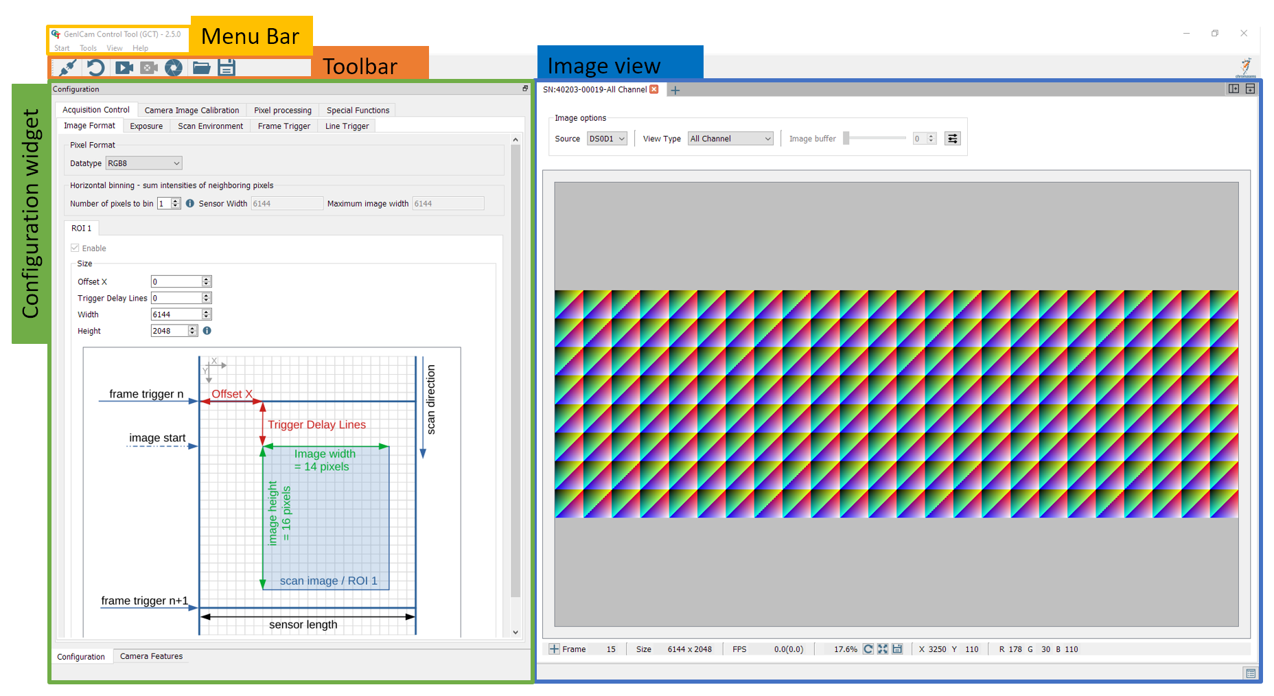
The software tool provides different panel elements that can be placed, resized, and docked freely within the GCT window. The GCT user interface starts after a successful connection with your camera. The window contains four main areas: the menu bar widget for general access, the toolbar widget for fast access to the most common functions, the image view widget where the image and all relevant information are displayed, and the configuration widget for the camera configuration.

Main window

Menu Bar

The Start Menu offers the following functions:

• Connect/Disconnect: Opens the device discovery widget or disconnects the camera, Connection and disconnection of Camera

• Start Grabbing: Starts continuous image grabbing

• Device description: Load and save XML file from/to the camera

• Settings: GCT setting options, GCT Options

• Exit: Close the GCT application

The Tools Menu offers the following functions:

• Calibration: Opens a camera calibration dialog, Create a black-reference (DSNU) and Create a shading-reference (PRNU)

• Maintenance Mode: Only for experts. Requires a password.

• Up/Download: Opens an Up/Download dialog, Up-Download

• Register Editor: Only for experts. Set or read register values in camera.

• Perform Adjustment A tool to help adjust the physical alignment of your camera.

The View Menu offers the following functions:

• Default view: Set the GCT widget arrangement to default

• Configuration Widget: Shows or hide the Configuration widget panel

• Feature Widget: Show or hide the Feature tree panel

• Image View: Show or hide the Image view window

• Message Log: Show or hide the Message Log widget

• Refresh Feature Tree: Refreshes the feature tree tab

The Help Menu offers the following functions:

• About: General information about GCT

• Open GCT Manual: Opens the GCT Manual

• System Information: Opens a system information dialog with an option to save the report

Toolbar

The Toolbar contains the following icons and their functions.

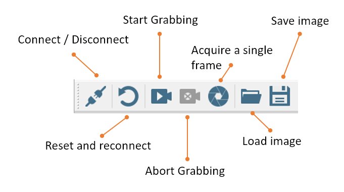
The Toolbar offers the following button functions:

• Connect/Disconnect: Opens the device discovery widget or disconnects the camera, Connection and disconnection of Camera

• Reset and reconnect: Resets the camera and reconnects

• Start Grabbing: Starts continuous image grabbing

• Abort Grabbing: Stops the image acquisition

• Acquire a single frame: Acquires a single frame

• Load image: Load an image from disk

• Save image: Save image to disk

Configuration widget

The Configuration widget provides two panels: Camera features, which is the GenICam parameter tree, and the configuration panel, which is a graphical representation of the GenICam parameter tree.

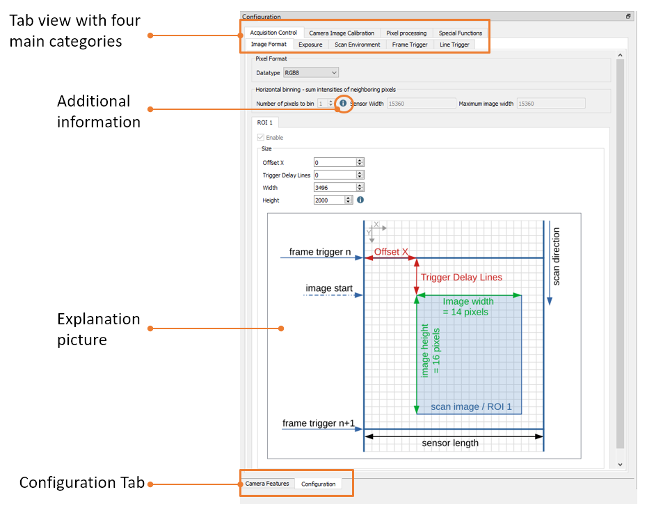
The following image shows the configuration panel of the configuration widget. The panel contains a tab view, from which four main categories can be selected. Each tab contains another tab view with subcategories. The content in each sub-tab view is scrollable.

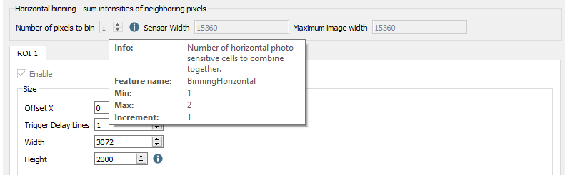
An info box or tooltip is shown when hovering over a parameter input field or the blue information icon.

The Camera Features tab contains the GenICam parameter tree, the user setup level, and an extra panel to set up the filter driver.

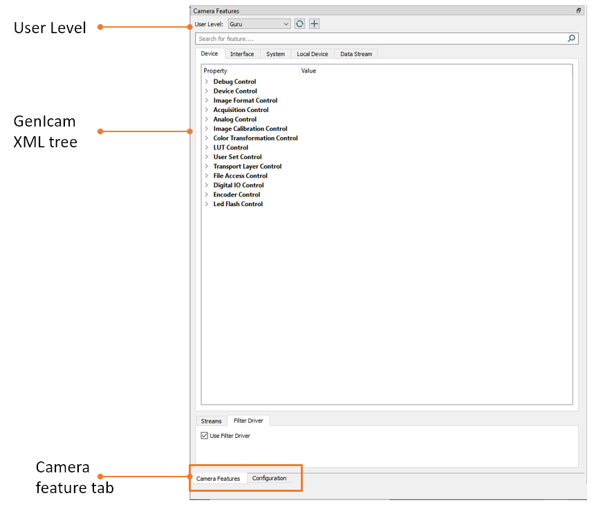
Image view widget

The image view widget shows the current image, image properties, acquisiton statistics and some functional tools to view image data in different forms.

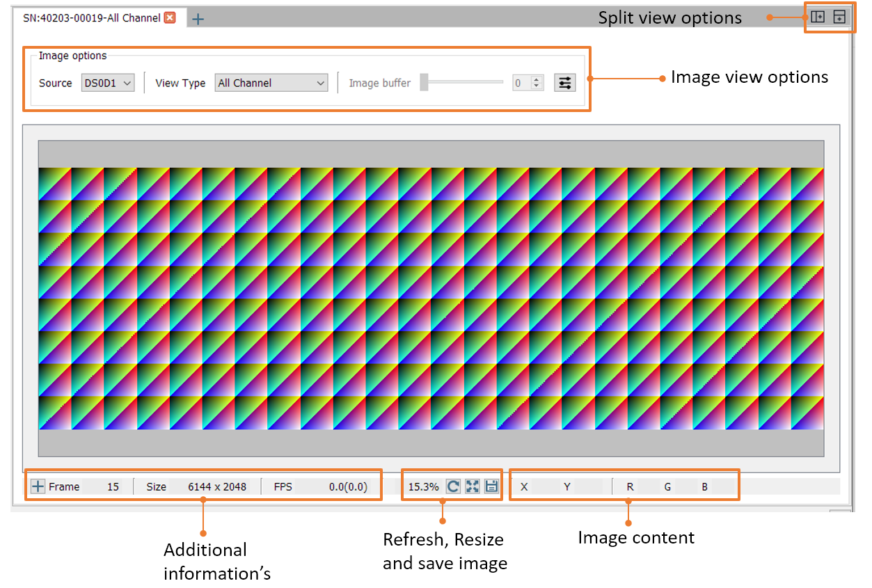
Split-view

The Split View option allows you to display multiple tabs side by side or on top of each other. As soon as two or more tabs are open you can select between the Horizontal Split-view and the Vertical Split view option.

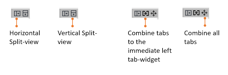
To end the Split-view you can choose between Combine tabs to the immediate left tab-widget or Combine all tabs.

The following image shows an example of the Horizontal Split-view.

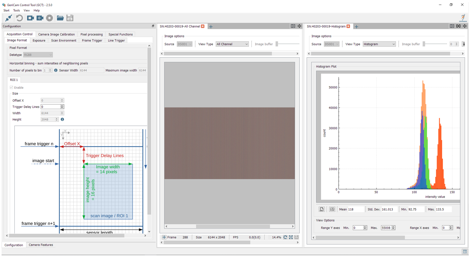
Image view options

Line plot view

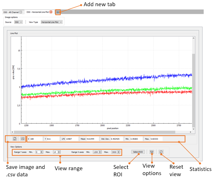
GCT can display a horizontal line plot in the image view widget. To add this feature, add a new tab by pressing the plus on the top. A popup window will open; select “Horizontal Line plot” under “View Type.”

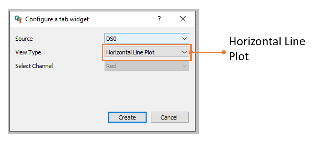
After this configuration, a new window will open as shown in the following figure.

Histogram view

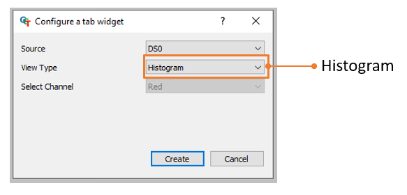
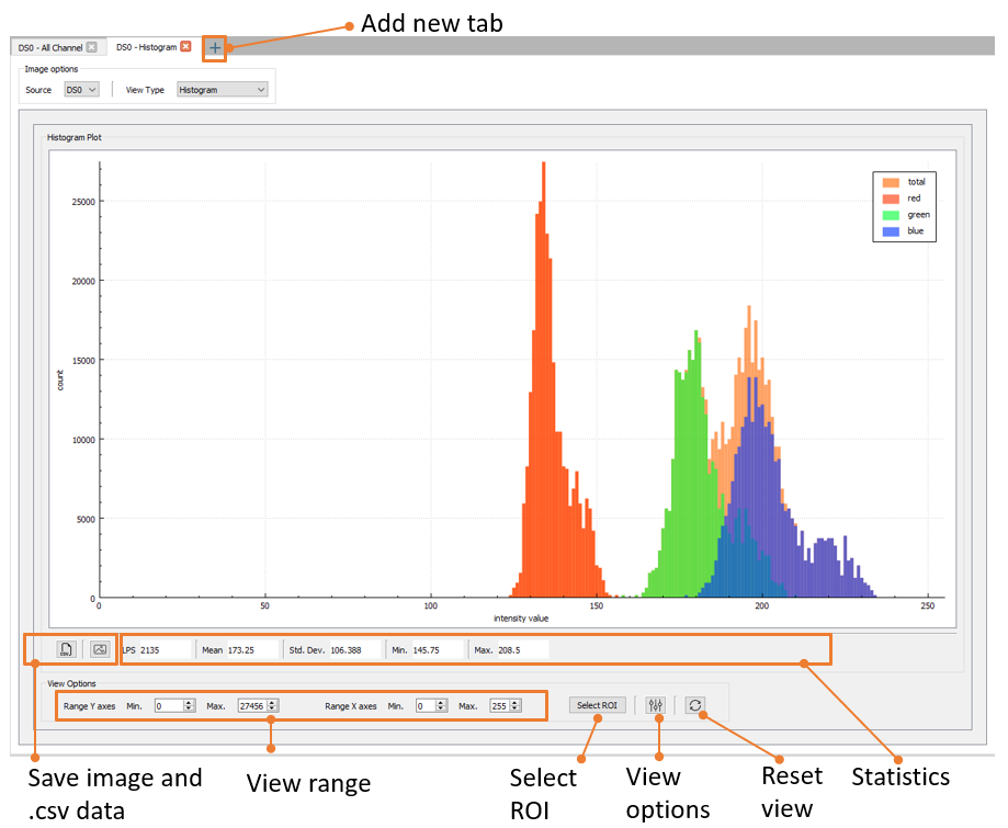
GCT can display a histogram of the image content in the image view widget. To add this feature, add a new tab by pressing the plus on the top. A popup window will open; select “Horizontal Line plot” under “View Type.”

After this configuration, a new window will open as shown in the following figure.

Single Channel

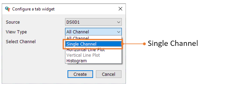
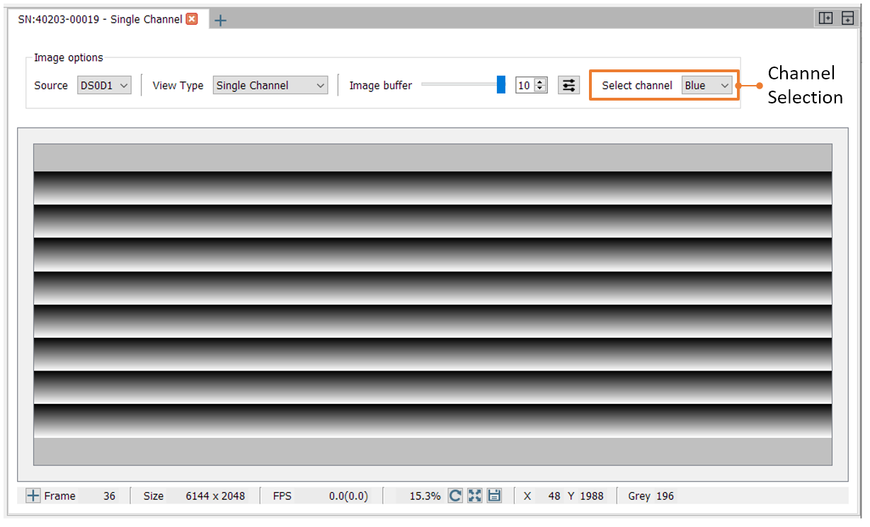
GCT can display only a single channel of the image content in the image view widget. To add this feature, add a new tab by pressing the plus on the top. A popup window will open; select “Single Channel” under “View Type.”

After this configuration, a new window will open as shown in the following figure.

Each Line Info Block analyzer

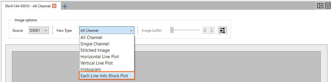
With GCT you can analyze the Each Line Info Block of the image content in the image view widget. To add this feature, add a new tab by pressing the plus on the top. A popup window will open; select “Each Line Info Block Plot” and then choose “Single Channel,” or change the View Type.

In this view, you can select four different plots. Navigate to Subview Type and select your feature of interest.

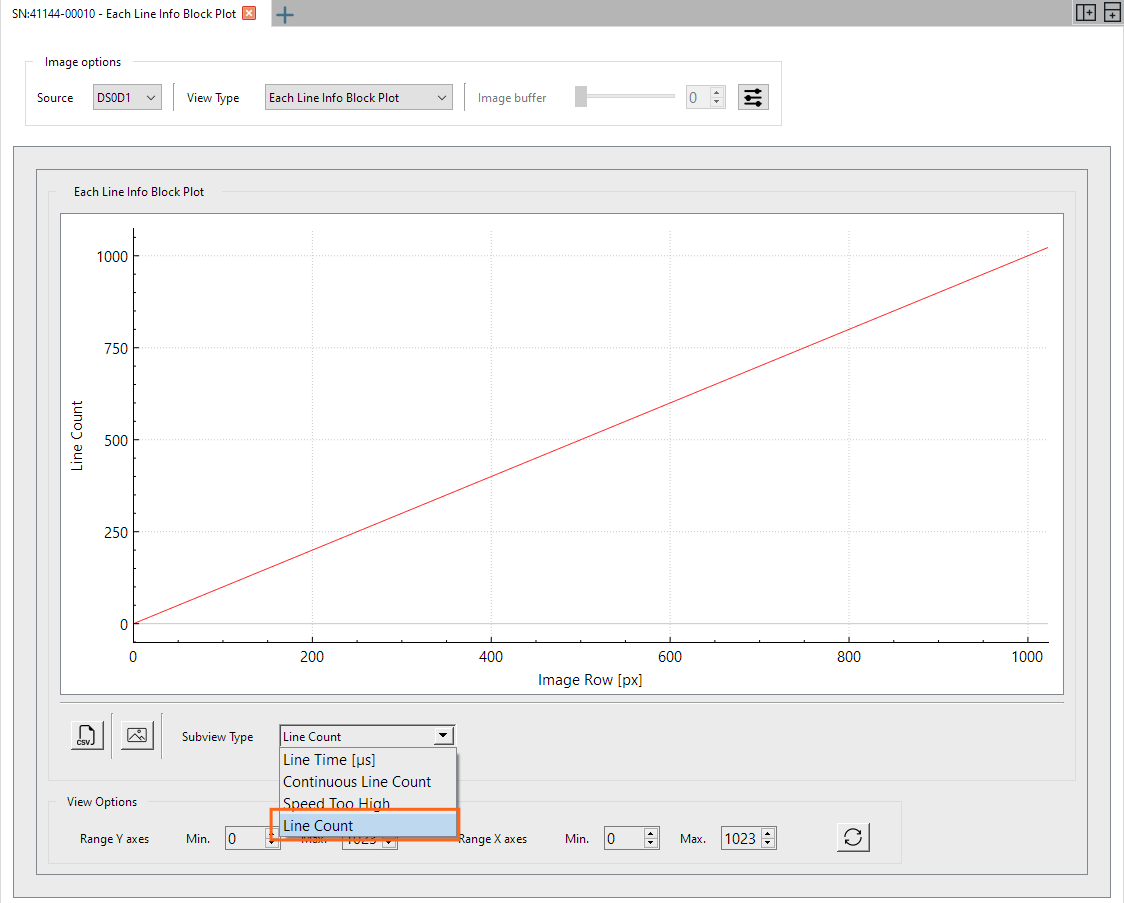
Image buffer

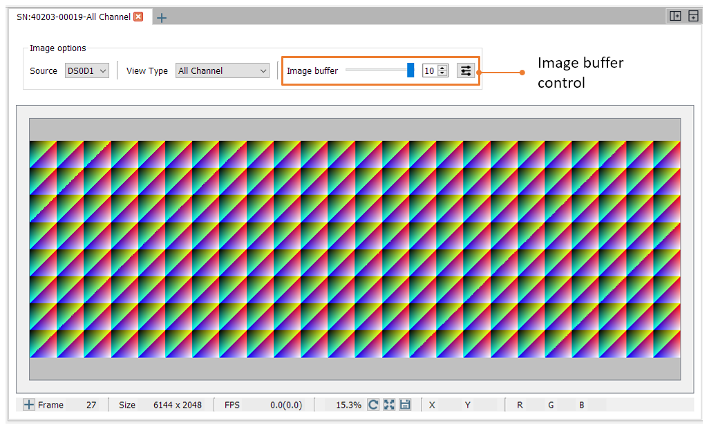
Multiple images can be buffered in GCT and displayed individually after stopping the acquisition. To enable this option, click on the right icon with the three sliders. A new window will open; check the Enable image buffer option.

Arrange / Rearrange widgets

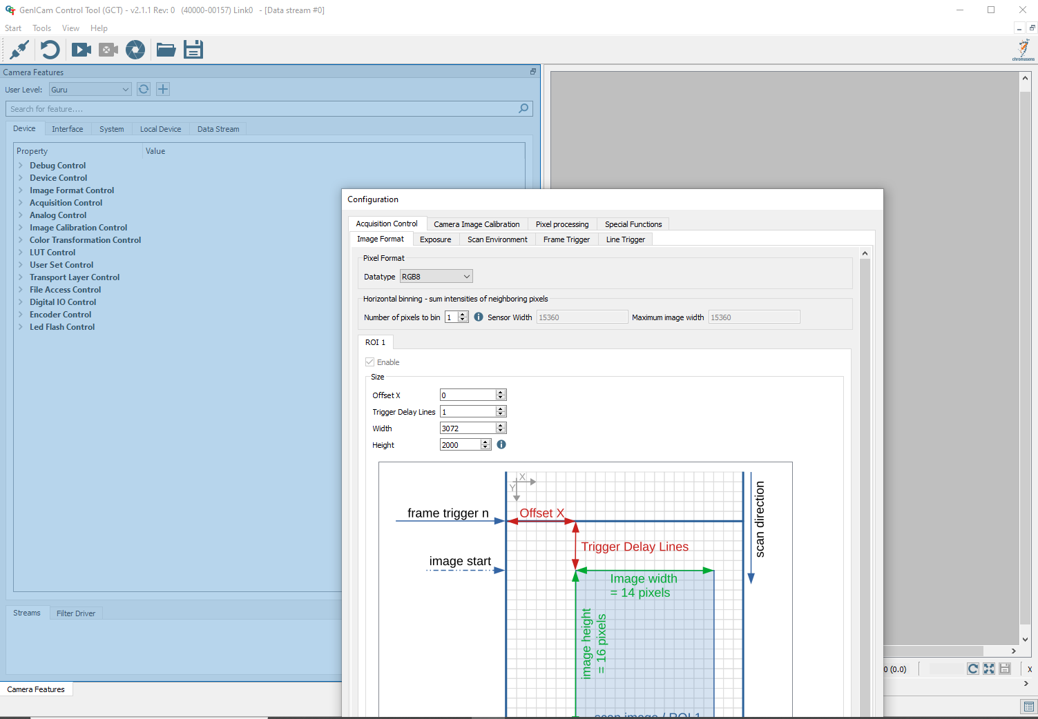
The software provides different widget elements that can be placed, resized, and docked freely within the GCT window. If you are using two monitors you can place, for example, the configuration widget on the second screen and the image view widget on the first screen.

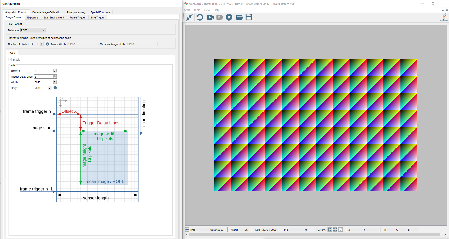
The software provides different widget elements that can be placed, resized, and docked freely within the GCT window. If you are using two monitors you can place, for example, the configuration widget on the second screen and the image view widget on the first screen.

Connection and disconnection of camera

Connecting the camera

To connect your camera:

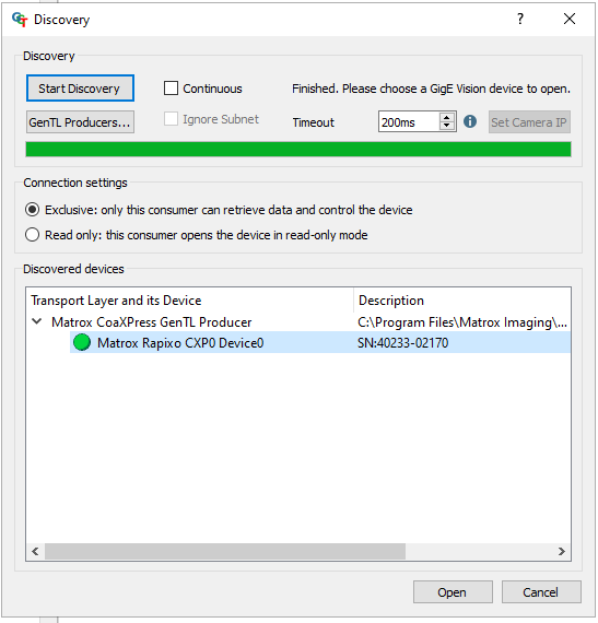
1. Click the Connect/Disconnect icon on the top left in the GCT Viewer toolbar.

2. The Discovery dialog opens. Click the Start Discovery button.

Note that camera initialization can take approximately 40 seconds.

Modifying features

GCT allows you to modify features in two different ways: The Configuration widget panel makes setting functions more convenient; special views show a set of related functions on which you can easily change these parameters. The camera feature panel allows you to edit the feature in the XML tree.

In the Configuration panel

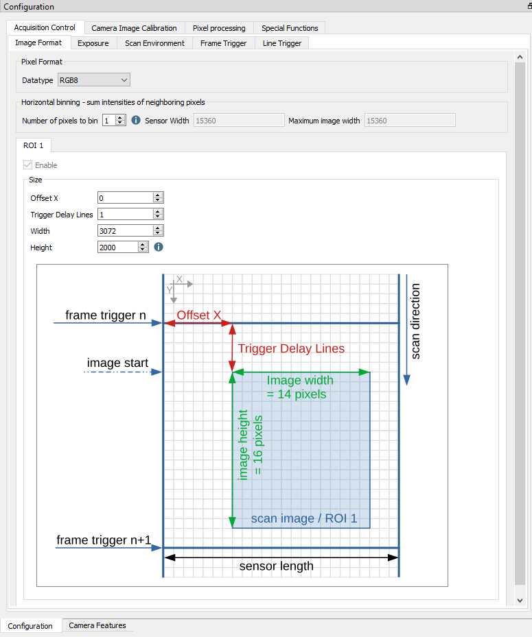
The view consists of four main tabs: Acquisition Control, Camera Image Calibration, Pixel Processing, and Special Functions. Each tab shows several subtabs.

The Acquisition Control tab, for example, shows five subtabs, which permit you to specify many features such as image format and trigger settings. Some features also have additional explanatory pictures.

In the camera feature panel (XML Tree)

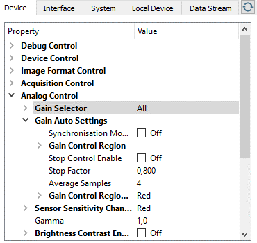
On the left side of the GCT window, features and their values are shown in a tree structure organized in feature groups. To show the features of a feature group, click on the arrow preceding the group name.

Showing feature details

Feature details can be displayed in the configuration panel and in the camera feature panel.

In the Configuration panel

In the configuration panel, the information is displayed when you move the mouse pointer over the parameter input field or the blue information icon.

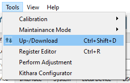
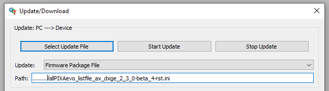
The Up-/Download dialog allows you to upload files from the PC to the camera—such as camera package files and user sets—and to download files from the camera to the PC. Supported file types and extensions depend on the camera type.

Uploading files to the camera

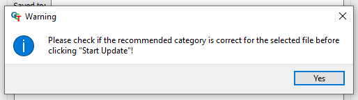
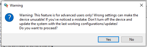
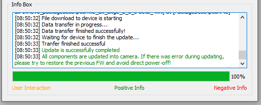
The Up-/Download dialog helps manage files on the camera. You can restore user settings, calibration files, and other file types that were previously downloaded from the camera.

Steps	Reference images
1. In the menu bar navigate to Tools. 2. Click Up-/Download or use the hotkey Ctrl+D.
The Update/Download wizard opens. 3. Click Select Update File and choose the file you want to upload, then click Open. 4. GCT shows a warning message. 5. Verify that the Type of your file matches the selected category in Update. 6. Click Start Update. 7. GCT shows a warning message. 8. Click Yes to start the upload. 9. Check the text in the Info Box: if the update was successful, it displays the green confirmation message “Update is successfully completed.”

Downloading files from the camera to the PC

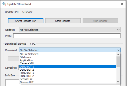
Firmware files, user sets, and other file types can be downloaded from the camera to the PC and saved locally.

Steps	Reference image
1. In the menu bar navigate to Tools. 2. Click Up-/Download or use the hotkey Ctrl+D.
The Update/Download wizard opens. 1. Click Download and select your file in the drop-down menu. 2. Click Download to. 3. Choose a folder, enter a file name, and click Save.

Updating the firmware

Warning

Irreparable damage to the camera

If the camera ist powered down during firmware update it may get into a non-functional state. Recovery may not be possible.

The following video shows how to update the firmware:

Creating a black-reference (DSNU)

Create a black-reference with DSNU.

1. Switch off the illumination.

2. Cover the lens with a black or dark piece of cardboard or plastic. No light may reach the sensor.

3. In the menu bar navigate to Tools → Calibration.

4. Click Generate DSNU Reference.

The Generate DSNU Reference wizard opens.

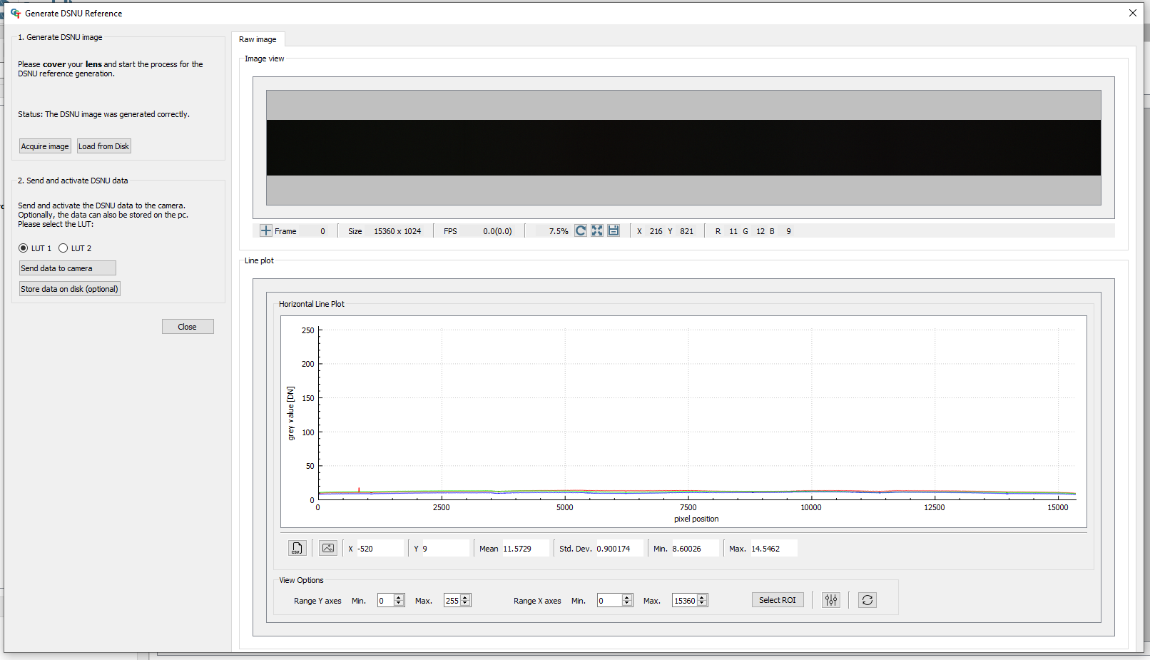
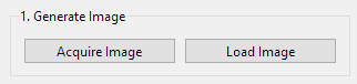
5. Click Acquire image to generate the DSNU directly from the camera, or click Load from Disk to load an image from the hard drive.

   Note

   Load from Disk:

   Make sure that the image has been taken with active image calibration mode by using the wizard.

The raw image and the line plot of the image is displayed.

Send the calculated DSNU to the camera:

6. Select LUT 1 or LUT 2.

7. Click Send data to camera. This activates the calibration LUT.

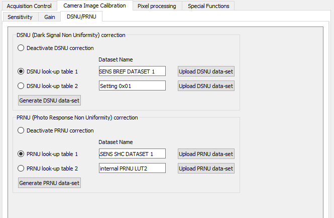
8. In the Configuration window, navigate to Camera Image Calibration → DSNU/PRNU.

9. Make sure that DSNU is enabled.

Creating a shading-reference (PRNU)

Note

Calculation of PRNU

The following equation describes the calculation of the PRNU:

Calibrated_Image = (Raw_Image - DSNU) / PRNU

PRNU = (PRNU_Image - DSNU) / Target_Value

• Calibrated_Image = Camera output with applied DSNU and PRNU

• Raw_Image = Camera output image without any correction

• Target_Value = Target Value of PRNU, default value is 255

• PRNU_Image = Acquired image of the white-reference

• PRNU = Photo response non-uniformity

• DSNU = Dark signal non-uniformity

Standard Method: PRNU reference generating (white diffuse surface)

Create a shading-reference with PRNU.

1. Place a moving white target. If using a stationary target, place it slightly out of focus.

Acquire an image:

2. In the toolbar click Acquire a single frame or click Start grabbing, wait until an image is displayed, click Stop grabbing.

3. In the menu bar navigate to Tools → Calibration.

4. Click Generate PRNU Reference.

The Generate PRNU Reference wizard opens.

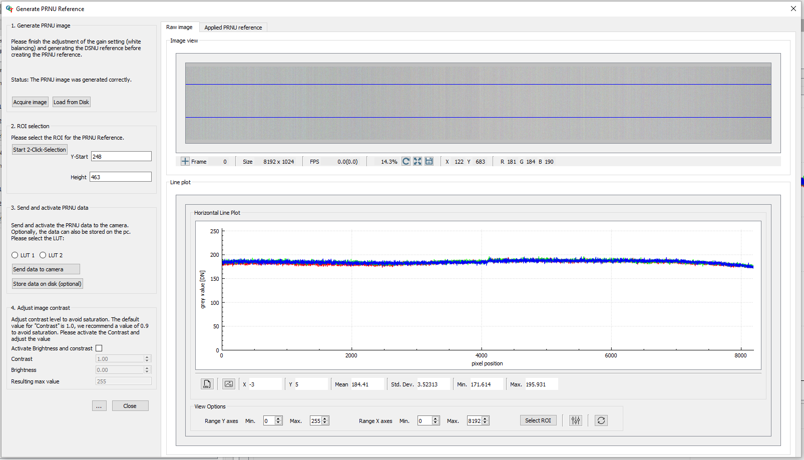
5. Click Acquire image to generate the PRNU directly from the camera, or click Load from Disk to load an image from the hard drive.

   Note

   Load from Disk

   Make sure that the image has been taken with active image calibration mode by using the wizard.

The raw image and the line plot of the image is displayed.

6. Click Start 2-Click-Selection.

7. Click on the image to select the ROI.

Send the calculated PRNU to the camera:

8. Select LUT 1 or LUT 2.

9. Click Send data to camera.

Activate brightness and contrast:

10. Select the Activate Brightness and contrast checkbox.

11. Set the contrast to 0.9.

Independent Method: PRNU reference generating channel independent

Note

This function is available as of GCT version 3.2.

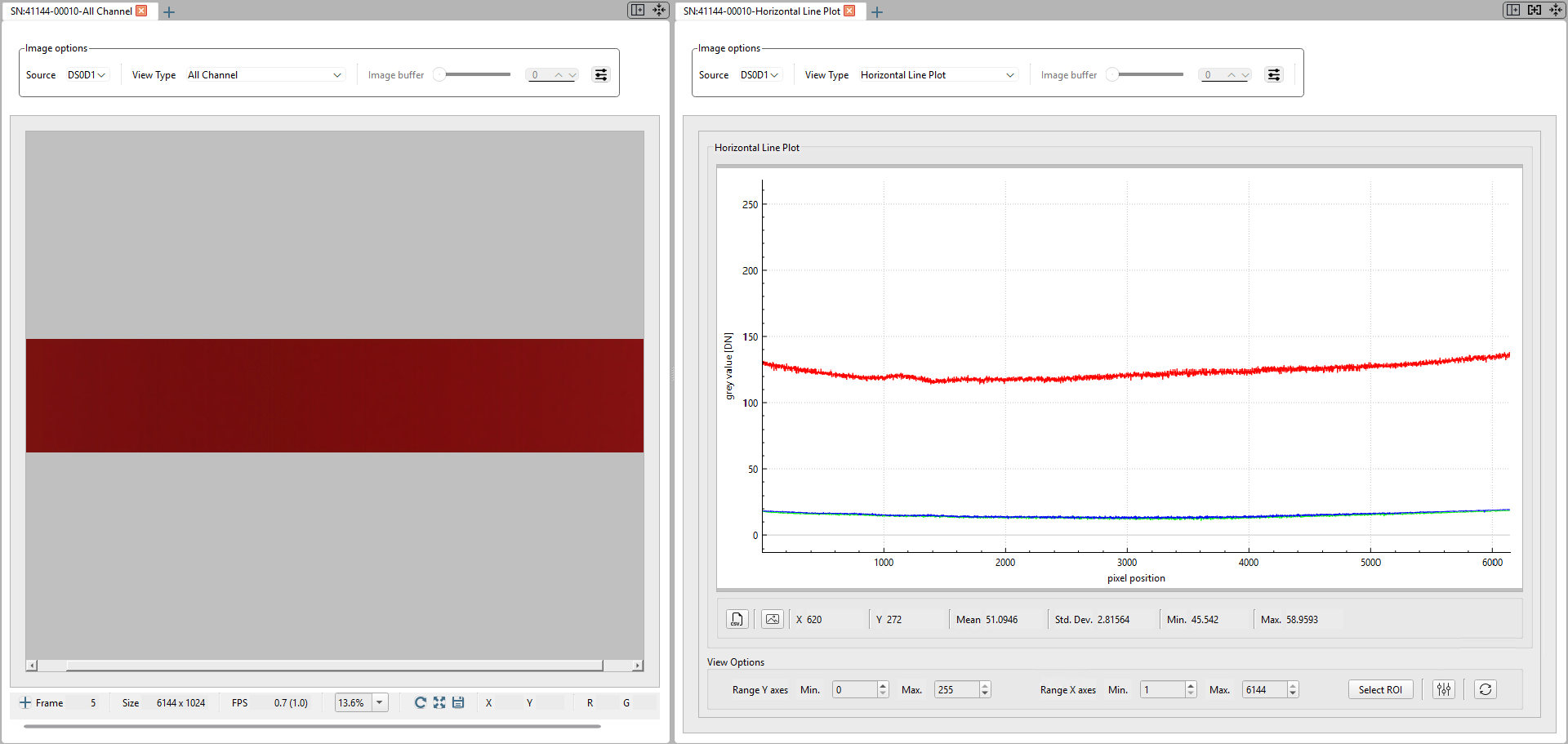
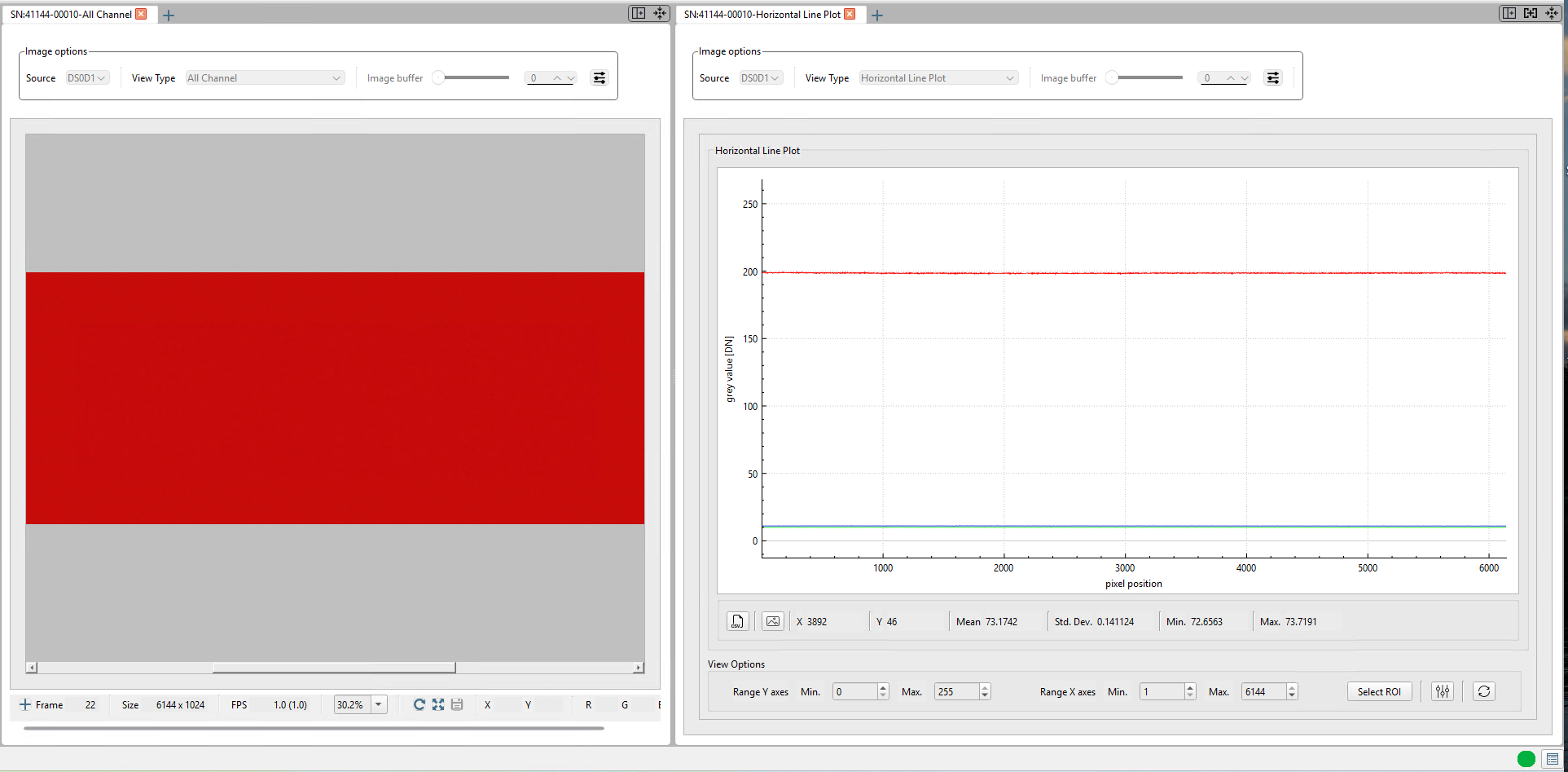
In this instance, the lighting arrangement is single-colored and is visible in the camera’s red color channel. The signals in the green and blue channels are quite minimal.

On the left of the image, you can observe the RGB image, while on the right, the profile of the horizontal line plot is displayed.

In this scenario, the result of the PRNU calibration should be a RED image exhibiting a uniform profile.

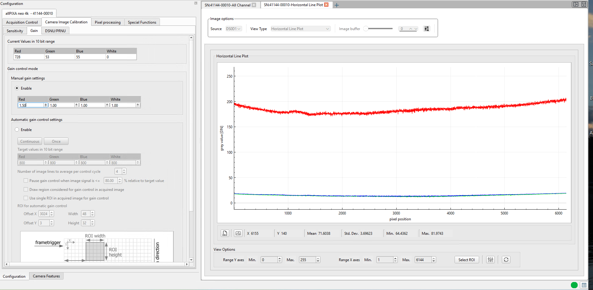
The “white balancing” process in the Independent calibration technique varies. The gain level needs to be modified for each specific gain. In this case, the Gain is solely applied to the Red channel.

1. In the menu bar navigate to Tools → Calibration.

2. Click Generate PRNU Reference.

The Generate PRNU Reference wizard opens.

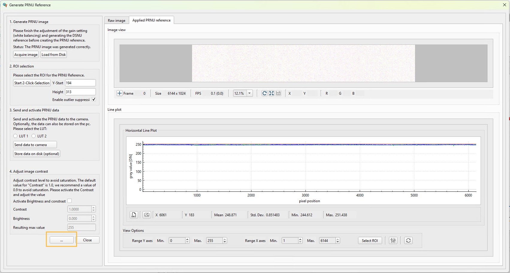
3. Click Acquire image to generate the PRNU directly from the camera, or click Load from Disk to load an image from the hard drive.

   Note

   Load from Disk Make sure that the image has been taken with active image calibration mode by using the wizard.

The raw image and the line plot of the image is displayed.

4. Click Start 2-Click-Selection.

5. Click on the image to select the ROI.

The view changed to the “Applied PRNU Reference”. This is the output of the Standard PRNU method. The image is very noisy.

6. Click on the button with the three dots …

7. The GUI changed and shows more options.

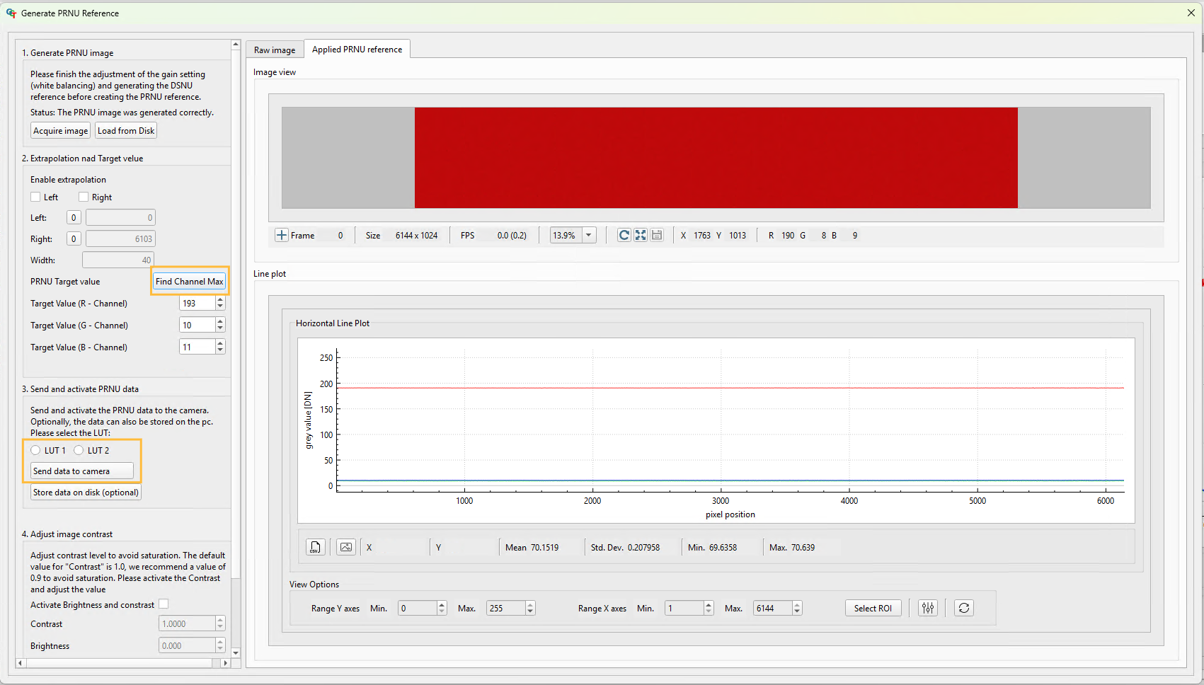
8. Click Find channel max — the PRNU algorithm will find the mean maximum value for each channel.

9. Change the Target Value, in this example Target value Red to 200.

Send the calculated PRNU to the camera:

10. Select LUT 1 or LUT 2.

11. Click Send data to camera.

Activate brightness and contrast:

12. Select the Activate Brightness and contrast checkbox.

13. Set the contrast to 0.9.

This image illustrates the results of the calibration process. It is a uniform image.

Extrapolation function

If the white reference does not cover the entire FOV, the extrapolation function can be used to generate it. In this case, a straight line is fitted to the gradient. Therefore follow the description below.

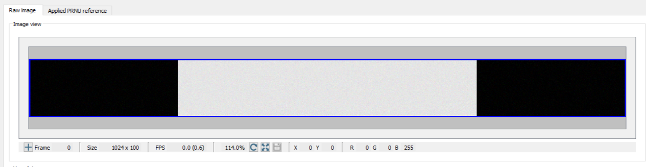
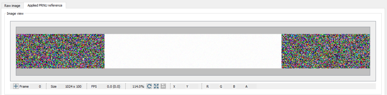
The images below show the raw image and the Applied PRNU reference without the extrapolation function. In the area with low image content, the Applied PRNU reference shows some artifacts.

1. Select the ROI by using Start-2-Click-Selection.

2. Press the button with the three dots on the bottom.

3. Enable your option, in this example the left extrapolation.

4. Select the start position of your extrapolation. The width defines the area where the extrapolation is created. From the start position to column 0, the extrapolation is applied.

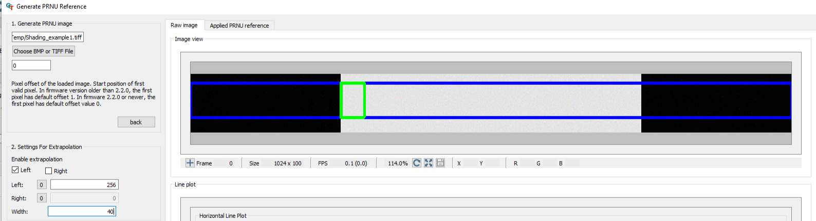
5. Check the applied PRNU in the Applied PRNU reference tab.

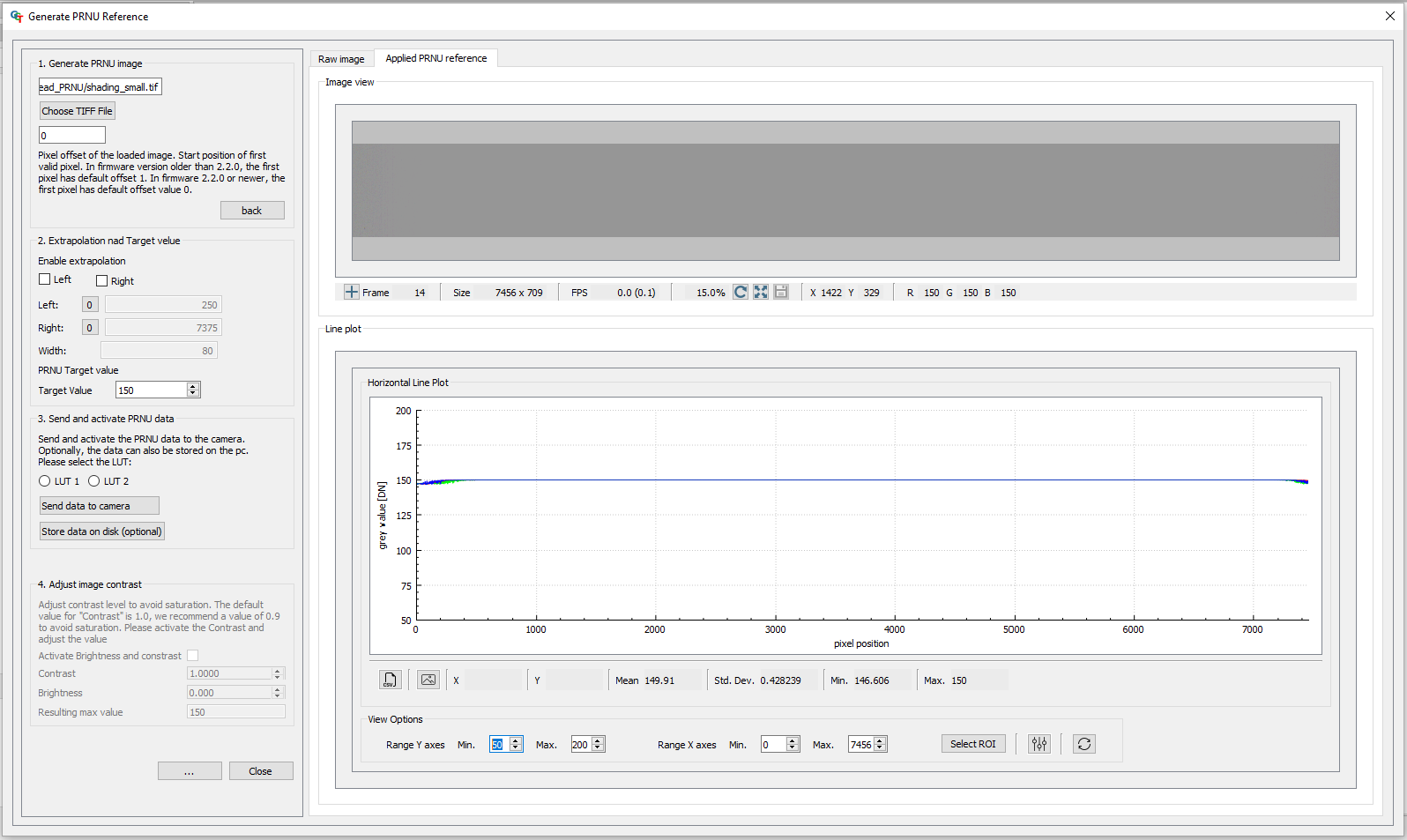
Target Value

The Target Value limits the maximum intensity of your Calibrated_Image.

Note

Make sure that the values of your PRNU_Image are smaller than your Target_Value.

1. Press the button with the three dots on the bottom.

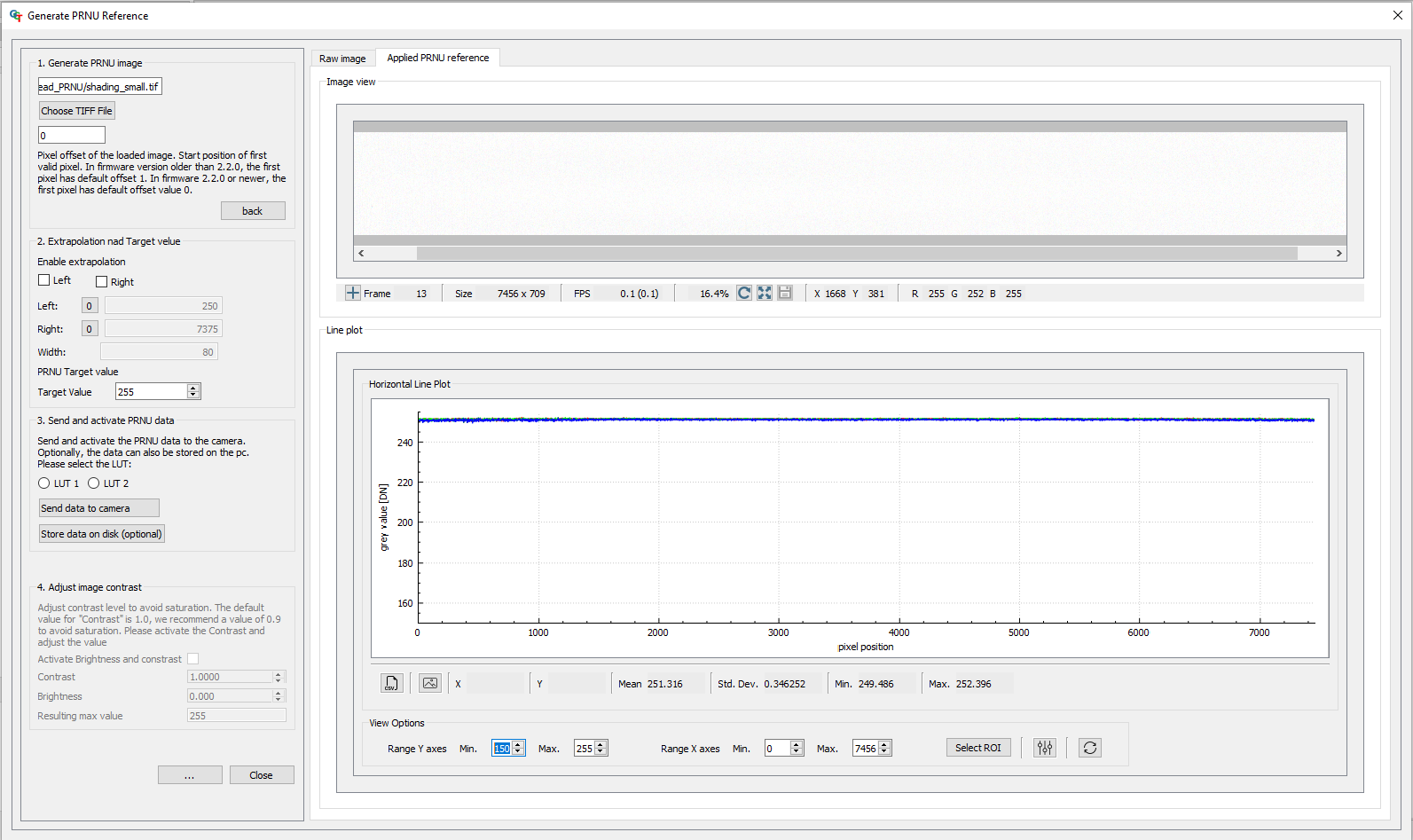
2. Change the Target Value.

3. Check the applied PRNU in the Applied PRNU reference tab.

Color metric

Delta E

Interpretation of the delta E values

Delta Value	Human Perception
0.0 – 1.0	Not or hardly perceptible
1.0 – 2.0	Perceptible by experienced observers
2.5 – 3.5	Perceptible even by inexperienced observers
3.5 – 5	Clear color difference
5.0 and higher	Large color difference

User level

Each camera contains an XML file specifying the available camera features. When GCT connects to the camera, it loads the XML file and shows the features as a tree structure.

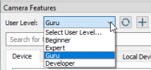
Each feature has a visibility level. While all features are displayed for user-level Developers, many advanced features are hidden for user-level Beginner.

The User Level is shown above the feature area of the Camera Features widget. To modify the user level, click the displayed User Level, and then click the desired level:

Show message log

To show the message log, click Message Log on the View menu or click Show message log window in the bottom right corner of the GCT window. A Message Log area is then shown below the image area:

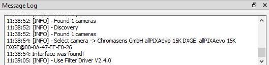
To copy messages to the clipboard, mark the messages, right-click on the selected messages, and then click Copy on the appearing context menu.

To copy all present messages, right-click on the Message Log area, click Select All on the appearing context menu, and then press Ctrl+C.

GCT options

To open the Options dialog box, click Options on the Start menu.

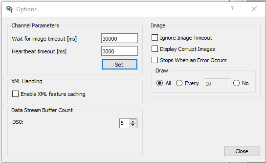
Option name	Default value	Description
Wait for image timeout	30000	If the next image is not received after the specified time, a timeout occurs. The value can be modified. When GCT is restarted, it is reset to 30000.
Heartbeat timeout	3000	Reads the value of GevHeartbeatTimeout from the camera (control channel).
Data Stream Buffer Count	5	Specifies the number of buffers used for each stream. The value should be at least 2 or 3.
Ignore Image Timeout	Not selected	Can be selected if the acquisition process should continue despite a timeout error.
Display Corrupt Image	Not selected	Can be selected if an image should be displayed despite missing data.
Stops If an Error Occurs	Not selected
Draw	All	Can be set to display every x frames, or to shut off display to reduce CPU usage.
Enable XML feature caching	Not selected	Ensures the actual value is retrieved directly from the camera instead of from a cached register.

The options (except Wait for image timeout and Heartbeat timeout) are saved in GCC.ini.

GCC ini file

The GCC.ini file, located at C:\Users\Public\Documents\Chromasens\GCT2, is automatically updated with the producer path, producer filename, and selected producer for discovery. Therefore, if discovery has already been executed, the GCC.ini file might look as follows in the [DefaultProducers] block:

• ProducerList contains the found CTI transport layer files.

• AdditionalSearchPath lists additional search paths for CTI files, which can be added by clicking Add Producer Path.

• SelectedProducerList contains the CTI transport layer files selected for the discovery process.